Subject analysis: Prune a statistics field from non-brain areas

A signal model has been fitted to FMRI session data:

fmrifit -v --stimulus-block letter --window 2 1 1 --id 2

The WLS optimisation in the fitting procedure uses a weighting scheme with non-null spatial extent. Thus, evaluating (i.e. fitting) an FMRI model close but outside of the actual brain of a subject will nevertheless result in »valid« parameter estimates. These »outside fits« can be detected post-hoc as they are naturally accompanied by a drastic drop in sample size.

By default, fmrifit will estimate a default data mask in standard space from the foreground/background difference saved in subject.session. If this mask still contains non-brain areas (and it is likely that it does), you may want to further prune the fitted parameter fields from these areas.

Fitting a brain mask: fmriprune

The command line programs fmriprune or fsl4prune can be used to generate brain masks and help in detecting these non-brain areas in the fit. Both commands will force a minimum number of observations to be available around each grid point either by setting a user defined hard lower bound for the minimum:

fmriprune -v --threshold 1800

Or by setting the lower bound to a given fraction of the maximum available measurements around a point:

fmriprune -v --fraction .7

The options --threshold and --fraction are exclusive and the default is --fraction .6842. The generated brain mask is directly saved into the file subject.fit.

Fitting a brain mask: fsl4prune

The difference between fmriprune and fsl4prune is that the latter also contains a wrapper to the FSL command line tool BET:

fsl4prune -v

The wrapper is equivalent to the following:

fmriprune --fit subject.fit

from fmristats import *
result = load('subject.fit')
result.mask()
intercept = result.get_field('intercept', 'point')

from fmristats.nifti import image2nii
import nibabel as ni
ni.save(image2nii(intercept), 'intercept.nii.gz')

bet intercept.nii.gz mask.nii.gz -R

nii2image mask.nii.gz mask.image

from fmristats import *

result = load('subject.fit')
mask = load('mask.image')

result.population_map.set_vb_mask(mask)
result.save('subject.fit')

Fitting a brain mask: Python

The Python interface gives you further control for defining brain masks. Load a statistics field to Python:

from fmristats import *
result = load(path_to_fit)

The statistics fields:

import matplotlib.pylab as pt
from fmristats.plot import picture

a0 = result.get_field('intercept','point')
b0 = result.get_field('task','point')
t0 = result.get_field('task', 'tstatistic')

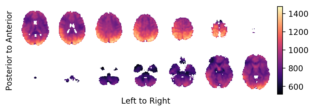
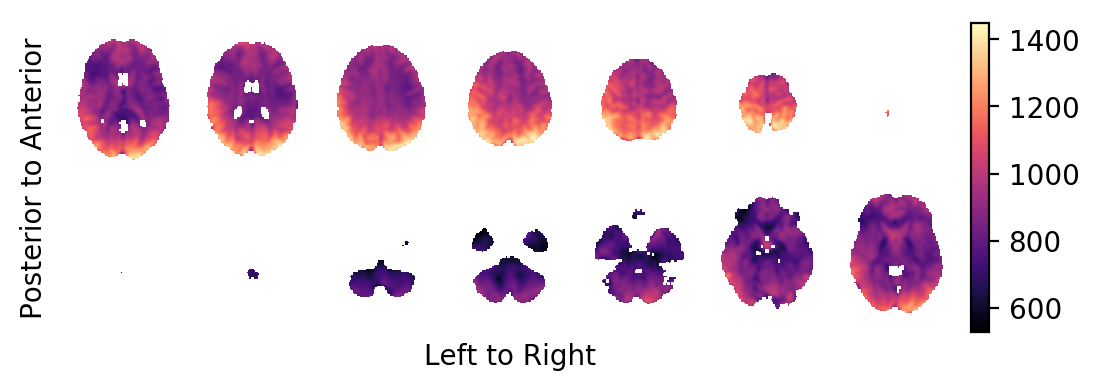
The intercept:

picture(a0,interpolation='bilinear')

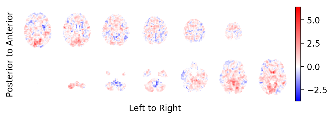
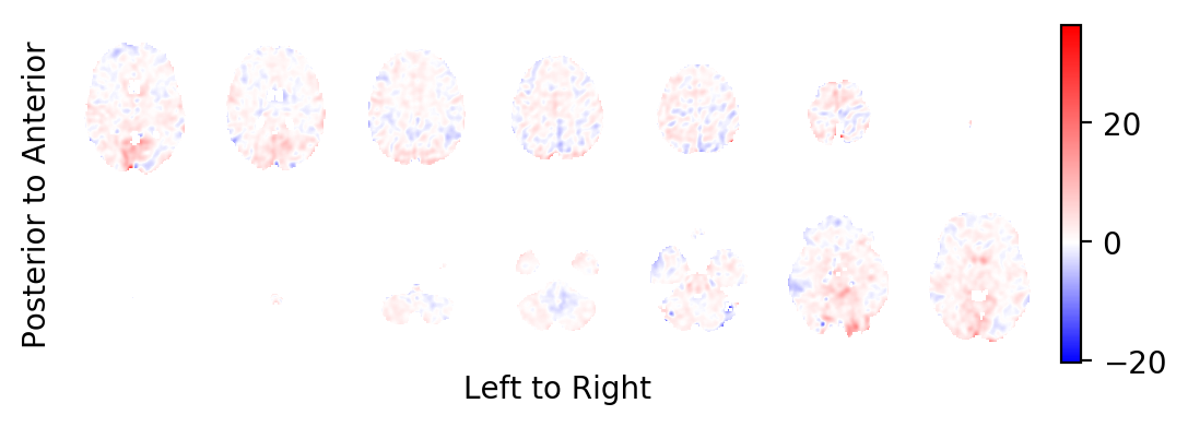
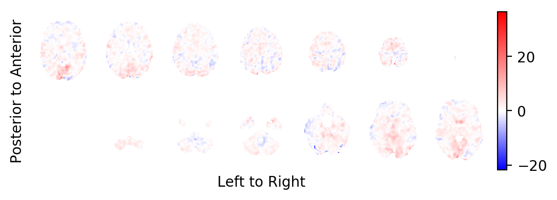
The BOLD effect field:

picture(b0,interpolation='bilinear')

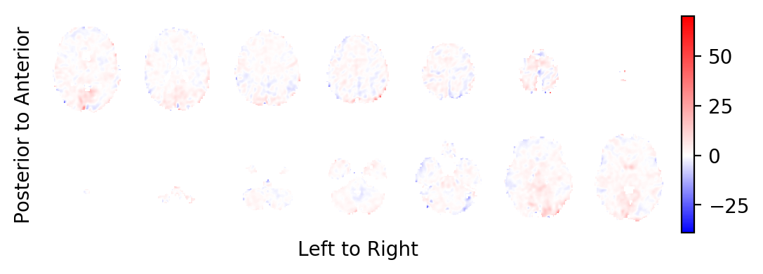
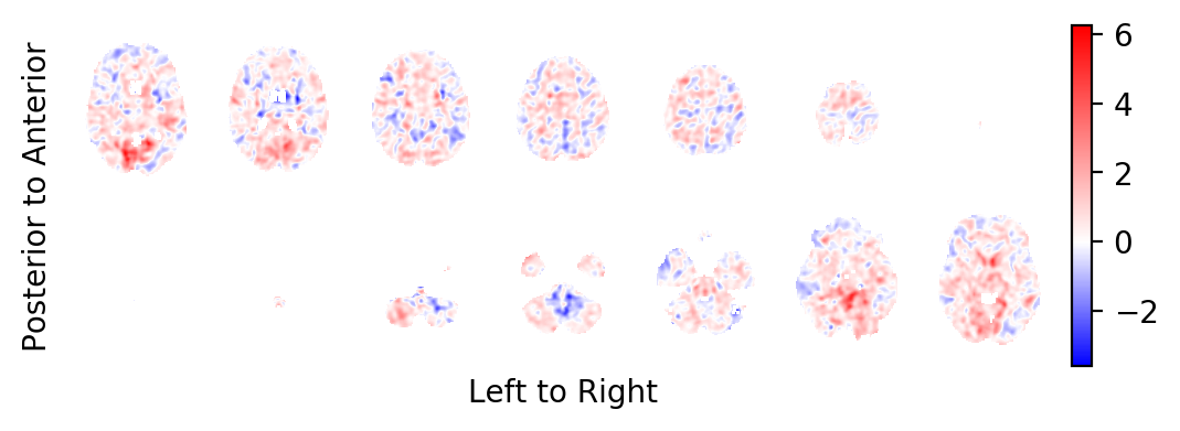
The t-statistics field:

picture(t0,interpolation='bilinear')

Most notably, you should realise that the task related BOLD effect field looks very faint: In contrast to some very large and strong effects on the periphery of the brain (strong in absolute effect size, not in significance), the BOLD effects within the brain are very weak. This is a sign that these effects are likely the result of small errors in the estimated head movements of the subject and not the result of BOLD changes in the MR signal. You want to prune the statistics field from these areas.

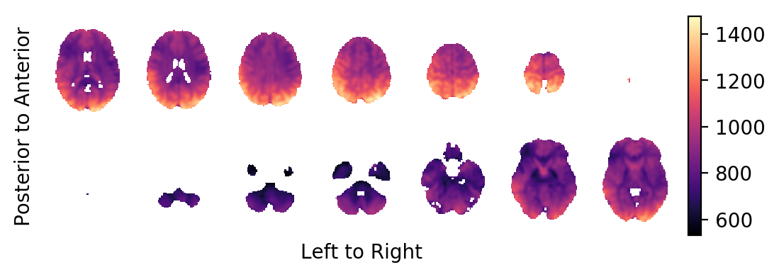
By threshold

Set a threshold for the minimum number of observations that should be available for fitting; set this number to a proportion of the maximum available sample size.

gf = result.get_field('df')
proportion_df = .6
threshold_df = int(proportion_df * np.nanmax(gf.data))

print('Lower threshold for the degrees of freedom: {:d}'.format(
    threshold_df))

Lower threshold for the degrees of freedom: 2263

Apply the threshold:

result.mask(gf.data >= threshold_df)

a0 = result.get_field('intercept','point')
b0 = result.get_field('task','point')
t0 = result.get_field('task', 'tstatistic')

The intercept:

picture(a0, interpolation='bilinear')

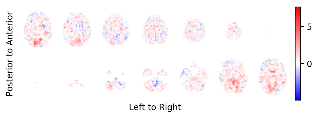
The BOLD effect field:

picture(b0, interpolation='bilinear')

The t-statistics field:

picture(t0, interpolation='bilinear')

And indeed, the task related BOLD effect field looks less faint.

By BET

You map also apply BET on the intercept.

from fmristats.fsl import bet

template = bet(
        intercept = a0,
        intercept_file = 'interim-results/intercept.nii.gz',
        mask_file = 'interim-results/intercept-mask.nii.gz',
        cmd='fsl5.0-bet',
        verbose = 2)

fsl5.0-bet
  interim-results/intercept.nii.gz
  interim-results/intercept-mask.nii.gz
  -R

Apply the mask:

result.mask(template.get_mask())

a0 = result.get_field('intercept','point')
b0 = result.get_field('task','point')
t0 = result.get_field('task', 'tstatistic')

The intercept:

picture(a0,interpolation='bilinear')

The BOLD effect field:

picture(b0,interpolation='bilinear')

The t-statistics field:

picture(t0,interpolation='bilinear')