Getting to know fmristats

Various command line tools provide access to most of fmristats’ functionality. In particular fitting a model to subject data is well covered by command line tools.

Before you start, a small but important warning: more »traditional« approaches to FMRI data analysis recommend and even encourage user to spatially smooth data prior to the statistical analysis and to also apply motion or slice timing corrections. In fmristats, spatial smoothing is an integral part of the model fitting process itself. Therefore, when using fmristats:

Warning

• DO NOT alter your images.
• DO NOT perform any kind of motion correction.
• DO NOT correct for slice timing differences.
• DO NOT smooth your data.

Your statistical analysis will benefit, you will gain power, and you will be rewarded with valid statistical tests.

To fit a signal model to the FMRI session data of a subject, you will need to:

1. Define the stimulus, conditioning, or paradigm of the session, i.e. you will need to provide the on- and offsets (or durations) of the task blocks.
2. Separate the foreground from the background in the 4D FMRI image.
3. Estimate (or provide) the locations, positions, and tilts of the subject’s head in the scanner during acquisition, i.e. you need to estimate the subject’s head movements in the scanner.
4. Estimate the diffeomorphism that relates the subject brain to a given template.
5. Define and fit the model to your data.
6. Prune the fitted statistics field from non-brain areas.

This tutorial will go through each of these steps.

Formally, the analysis of an FMRI session is the juggle between three spaces. There is the scanner space \(S\) equipped with a coordinate system (read: basis vectors) with reference to the MRI scanner. There is the subject reference space \(R\) equipped with a coordinate system with reference to the head of the subject (in other words, the coordinate system of \(R\) stays fixed with the subject’s head and the coordinate system moves with the head during acquisition). And finally, there is a standard space \(M\). For the standard space, we assume that for a given template image \(m\) in \(M\), the image of the subject head is diffeomorph to m. These spaces are connected by rigid body transformations \(ρ_t\) and a diffeomorphisms \(ψ\):

\[M {\xrightarrow ψ {}} R {\xrightarrow {ρ_t}{}} S.\]

The diffeomorphism \(ψ\) maps the template brain onto the subject brain in \(R\), and the rigid body transformations \(ρ_t\) map the brain in \(R\) to the position of the brain within the scanner at time \(t\) of the acquisition sequence.

All current standard approaches to the statistical analysis of FMRI data (FSL, SPM, AFNI, ANTS) first pull the data from \(S\) to M and perform the statistical analysis in \(M\). (This is why there is so much pre-processing needed by these approaches.) This is very different to the approach that is favoured here. In fmristats, the analysis is performed with the actual collected data in \(S\). This has been made possible by the recent development of the model based (MB) estimator that is described in detail here.

1. Stimulus files

Subjects in an FMRI study are presented with various stimuli during data acquisition. The following will define a two-block task design labelled HFM for subject 42 in a study called foo measured on the 1st of November, 2015 at 1:54 pm.

fmriblock --stimulus subject.stimulus \
    --cohort foo \
    --id 42 \
    --datetime 2015-11-01-1354 \
    --paradigm HFM \
    --namex shapes \
    --onsetsx 2 84 166 248 330 \
    --durationsx 30 \
    --namey faces \
    --onsetsy 37 119 201 283 \
    --durationsy 44 \
    --verbose

This saves the stimulus design to a file subject.stimulus. The control block has been labelled shapes, the stimulus block has been labelled faces (as you may have guessed, the stimulus paradigm in this example is a face-shape-matching). You may query information about the just created stimulus design by calling fmriinfo on the file:

fmriinfo subject.stimulus

Alternatively, you may first create a single subject study for the subject:

fmristudy -v -o foo.study \
    --cohort foo \
    --id 42 \
    --datetime 2015-11-01-1354 \
    --paradigm HFM \
    --single-subject subject

The string that is provided to --single-subject will be used as a prefix to all files created by fmristats command line tools: If you call fmriblock as:

fmriblock -v \
    --namex shapes \
    --onsetsx 2 84 166 248 330 \
    --durationsx 30 \
    --namey faces \
    --onsetsy 37 119 201 283 \
    --durationsy 44 \

This is equivalent to the former.

Almost all fmristats command line tools will search for the existence of a .study-files in the current directory and use any information that is provided in the file. In fact, fmriblock will traverse upwards in the file hierarchy (by default up to six levels but no further than the home directory of the user) and look for available studies.

Entering the on- and offsets of stimulus designs by hand is inefficient; in particular if you are planing to analyse a large number of subjects with potentially varying onsets. If your presentation software supports MATLAB-coded logfiles of the stimuli in the same format as described in Section 8.3 of the SPM Manual (see page 65), you can used mat2block to parse these files:

mat2block -v --mat subject.mat

Use -v/--verbose to increase verbosity of any fmristats command line tools.

2. Session files

Data import in fmristats is handled by Nibabel, allowing a flexible import from various formats for FMRI data; and this includes the popular Nifti1 format. You can create Nifti1-files from DICOM by using dcm2nii with all the default settings:

option	description
4D=1	“will generate 4D files (FSL style)”
SingleNIIFile=1	“will create .nii files (FSL style)”
Gzip=1	“will create compressed .nii.gz files (FSL style)”
SPM2=0	“headers will be in NIfTI (SPM5/FSL)”

If you save the 4D-image in subject.nii.gz, then nii2session will create an FMRI session file for you:

nii2session \
    --nii subject.nii.gz \
    --epi-code 3 \
    --detect-foreground -v

The session file is saved to subject.session. In case you have not created the above foo.study, this call in equivalent to:

nii2session --session subject.session \
    --nii subject.nii.gz \
    --stimulus subject.stimulus \
    --epi-code 3 \
    --detect-foreground -v

As the option --detect-foreground suggests, this will also run a foreground detection algorithm on the image.

The argument --epi-code 3 codes the direction in which the EPI have been measured during data acquisition. The direction is coded as follows:

EPI code	direction
-3	superior to inferior
-2	anterior to posterior
-1	right to left
1	left to right
2	posterior to anterior
3	inferior to superior

You may also provide more meta data to the call.

nii2session --session subject.session \
    --cohort foo \
    --id 42 \
    --datetime 2015-11-01-1354 \
    --paradigm HFM \
    --nii subject.nii.gz \
    --stimulus subject.stimulus \
    --epi-code 3 \
    --detect-foreground -vvv

By default, files will not be overwritten. Use -f/--force to force the recreation of any files.

You may query information about any file that is created by fmristats by calling fmriinfo on the same.

fmriinfo subject.session

Output:

subject.session: session file

        Cohort:   foo
        Subject:  42
        Date:     2015-11-01-1354
        Paradigm: HFM

        EPI code: 3

        Type of stimulus: block design
        Block number: 2
        Block names:  ['shapes', 'faces']
        Number of onsets per block: {'shapes': 5, 'faces': 4}

        Resolution (left to right):          3.28 mm
        Resolution (posterior to anterior):  3.28 mm
        Resolution (inferior to superior):   4.18 mm
        Diagonal of one voxel:               6.25 mm
        Volume of one voxel:                45.00 mm^3
        Aspect 0 on 1:                       1.00
        Aspect 0 on 2:                       0.78
        Aspect 1 on 2:                       0.78

You may also provide more than one file to the call:

fmriinfo subject.stimulus subject.session

3. Reference maps

Subjects may tend to move their head in the scanner ever so slightly, which means that the tilt and position of the head during the FMRI session may change over time. For this reason, we need to track the subject head in the scanner, i.e. we need to find and estimate of its tilt and position at a given time point. Mathematically, head movements are affine transformations (rigid body transformations) that map from a space with a subject-specific coordinate system to the scanner space (or in other words from a coordinate system that is fixed with respect to the subject to a coordinate system that is fixed with respect to the scanner). Let us denote the subject reference space by \(R\) and the scanner space by \(S\). Then head movements are maps:

\[ρ_t : R \to S.\]

The inverse maps of the \(ρ_t\) are called the acquisition maps of scan \(t\):

\[ρ_t^{-1} : S \to R.\]

Hence, the acquisition map of scan \(t\) maps from scanner space to subject reference space.

The Python interface of fmristats is very flexible in how you may define the space \(R\) and the maps \(ρ_t\), and it is also easy to feed the fits of third party software to fmristats (such as fits from FSL-FLIRT or ANTS). Please see the documentation of the fmristats.reference module for more details.

On the command line, fmririgids provides a tool to fit a principal components model for estimating head movements:

fmririgids -v

And in case you are not working with the above foo.study, this call in equivalent to:

fmririgids -v --session subject.session --reference-maps subject.rigids

fmririgids gives you two options for defining the subject-specific coordinate system: you can either set the coordinate system in \(R\) to the average position of the head during sequence acquisition (this is the default), or to the position of the head within the scanner during a given scan cycle during the acquisition sequence:

fmririgids -vf --cycle 42

When running fmririgids, you may have already noticed that fmririgids also performs an outlier detection: The idea is to exclude scan cycles during which the subject shows severe movements. Scan cycles which are marked as outlying will not be used when fitting any model to the FMRI data. You will also not be able to set the reference coordinate system of a subject to a suspected outlying scan cycle. You can, however, provide fall back alternatives:

fmririgids -vf --cycle 42

Found study: ./foo.study
Read study: ./foo.study
Working directory changed to: /path/to/results
Process protocol entries sequentially
foo-0042-HFM: Read subject.session
foo-0042-HFM: Read subject.rigids
foo-0042-HFM: Lock: subject.rigids
foo-0042-HFM: Start fit of rigid body transformations
foo-0042-HFM: Detect outlying scans
foo-0042-HFM: All suggested reference cycles have been
                marked as outlying. Unable to proceed. Please specify a
                different scan cycle (using --cycle) as reference.
foo-0042-HFM: Unlock: subject.rigids

fmririgids -vf --cycle 42 84 32

Found study: ./foo.study
Read study: ./foo.study
Working directory changed to: /path/to/results
Process protocol entries sequentially
foo-0042-HFM: Read subject.session
foo-0042-HFM: Read subject.rigids
foo-0042-HFM: Lock: subject.rigids
foo-0042-HFM: Start fit of rigid body transformations
foo-0042-HFM: Detect outlying scans
foo-0042-HFM: Cycle 42 marked as outlying, using fallback.
foo-0042-HFM: Reference cycle is 84.
foo-0042-HFM: Save: subject.rigids

Some plots that may help in evaluating the fit of the head movements can be created by calling:

ref2plot -v

And in case you are not working with the foo.study file, this is equivalent to:

ref2plot --ref subject.rigids --rigids pcm -v

This will save various quality assessment figures to the directory figures/head-movements, but you may change this default location. Scan cycles which are marked as outlying will not be used when fitting any model to the FMRI data.

When looking at the plots, you may realise that the PC-method is quite sensitive and this sensitivity lead to potentially quite erratic head movement estimates. This suggests that it makes sense to flatten the estimates by e.g. a moving average window.

ref2plot -v --window-radius 5 --rigids pc5

A --window-radius of \(n\) means that the average rigid body transformation:

\[\bar ρ_t = \text{rigidmean} \{ ρ_s : t-n ≤ s ≤ t+n \}\]

is calculated and used as an estimate for the location and tilt of the brain at scan cycle \(t\).

You may also iterate the procedure. This effectively results in a weighted averaging of rigid body transformations in the neighbourhood of a scan.

ref2plot -v --window-radius 2 1 1 --rigids pc211

Note

The theory of the model based estimator suggests to use one estimate for the location and tilt of the subject head separately for each scan. Currently, the implementation does not live up to the possibilities provided by the theory: fmristats will use the same location estimate for all scans in a scan cycle. There is a rich literature on how to interpolate rigid body transformation (and in particular on how not to interpolate them). The issue appears to be non-trivial, and I will come back to it as soon as I have found a statistical sound method for rigid body transformation interpolation.

The Python interface, though, already allows to define rigid body transformation for each scan. If you have an estimate for each scan, you may want to use the Python interface. See fmristats.reference for details.

Note

In almost all quality assessement plots I have seen thus far, it appears that subjects seem to take a while before they »settle into the experiment«. This suggests that it it may be advantageous to pick a scan cycle as reference which lies well within the FMRI session. In particular you should probably not take the first scan in a session as the reference scan.

4. Population maps

As described above, an FMRI analysis is a juggle between three spaces: The space \(S\) (with a scanner-fixed coordinate system), the space \(R\) (with a subject-fixed coordinate system), and the so-called standard space \(M\). The reason for the introduction of the latter is that it is common to work not within a specific, individual coordinate system for each subject but to chart all brains with respect to a common standard.

Mathematically, we have to find a diffeomorphism \(ψ\) that maps a standardised template brain, say an image \(m\) living in \(M\), onto the subject brain that lives in \(R\):

\[ψ : M \to R\]

The map \(ψ\) together with \(m\) is called a PopulationMap in fmristats.

4.1 Setting standard space to an isometric image of the brain

If you are only interested in a single subject, you may set \(M\) to any isometric image of \(R\), i.e. to a standard space which preserves distances with respect to the subject. In other words, you may set \(ψ\) to any rigid affine transformation of your liking. This includes the special cases of setting:

• \(M=R\) and \(ψ = \text{id}_{MR}\) (the identity map form \(M\) to \(R\)),
• \(M=ρ_{t_0}[R]\) and \(ψ = ρ_{t_0}^{-1}\) for any scan \(t_0\) of your choice,
• \(M=\bar ρ[R]\) and \(ψ = \bar ρ^{-1}\) for the »average« rigid body transformation.

fmripop -v

This sets \(M\) to the average position of the subject head in the scanner (\(M=\bar ρ[R]\) and \(ψ = \bar ρ^{-1}\)).

fmripop -v --cycle 100 --population-map subject-100.popmap

This sets \(M\) to the image space of \(ρ_{100}\) (\(M=ρ_{t_0}[R]\) and \(ψ = ρ_{t_0}^{-1}\) for \(t_0 = 100\).)

fmripop -v --cycle 42 84 --population-map subject-id.popmap

In case you chose the same scan cycle as you have chosen in fmririgids, this corresponds to setting \(M=R\) and \(ψ = \text{id}_{MR}\).

All three calls create a dummy template in \(M\) with a default resolution of (2 mm x 2 mm x 2 mm). You may change this default by manually setting the --resolution:

fmripop -v --resolution 3.8 --pop subject-low-resolution.popmap

If you set the resolution to »0«, the resolution of the acquisition grid of the FMRI session will be used.

fmripop -v --resolution 0 --pop subject-native-resolution.popmap

4.1 Setting standard space to the domain of a template

Say you have given a template in some standard space:

nii2image --name mni152 \
    /usr/share/data/fsl-mni152-templates/MNI152_T1_2mm_brain.nii.gz \
    template.image

nii2image --name mni152-background \
    /usr/share/data/fsl-mni152-templates/MNI152_T1_2mm.nii.gz \
    background.image

Then you need to find a diffeomorphisms \(ψ\) from the domain \(M\) of the template to the reference space \(R\) of the subject.

ANTS

fmristats contains a wrapper to ANTS’ antsRegistrationSyNQuick.sh:

ants4pop -v --cycle 42 84 \
    --population-map subject-mni152-ants.popmap \
    --vb-image template.image \
    --vb-background-image background.image

Make sure that you provide the same arguments to --cycle as you have provided to fmririgids, since this assures that the diffeomorphism in subject-mni152.popmap maps to the same space as the acquisition maps in subject.rigids (the domain of the reference maps).

You can query information about the created population map by calling:

fmriinfo subject-mni152-ants.popmap

In case you have set the subject reference space \(R\) to the average position of the subject brain in the scanner (see section 3. Reference maps), then you need to provide ants4pop with an estimate of an »average« brain in \(R\); for example, a fit of a signal model in \(R\) (we haven’t covered fitting a model, yet):

ants4pop -v --fit subject.fit
    --pop subject-mni152-to-average-brain.popmap \
    --vb-image template.image \
    --vb-background-image background.image

FNIRT

If you are using FNIRT to fit the respective diffeomorphism \(ψ: M \to R\), then you may use the wrapper tool fsl4pop to parse the spline coefficients file that has been created by FNIRT.

fsl4pop -v --cycle 42 84 \
    --population-map subject-mni152-warpcoef.popmap \
    --vb-image template.image \
    --vb-background-image background.image \
    --fnirt-spline-coefficients custom-warpcoef.nii.gz

If you do not provide a file to --fnirt-spline-coefficients, then fsl4pop will call FNIRT with all the default options in order to fit the spline coefficients.

fsl4pop -v --cycle 42 84 \
    --population-map subject-mni152-fnirt.popmap \
    --vb-image template.image \
    --vb-background-image background.image

The wrapper fsl4pop does, however, allow you to modify the call and provide FNIRT with custom configuration files. Please have a look at fsl4pop -h for details.

Again, make sure that you provide the same arguments to --cycle as you have provided to fmririgids. This assures that the diffeomorphism in subject-mni152-by-fnirt.popmap maps to the same space as acquisition maps in subject.rigids (the domain of the reference maps in subject.rigids).

You can query information about the created population map by calling:

fmriinfo subject-mni152-fnirt.popmap
fmriinfo subject-mni152-warpcoef.popmap

In case you have set the subject reference space \(R\) to the average position of the subject brain in the scanner (see section 3. Reference maps), then you need to provide fsl4pop with an estimate of an »average« brain in \(R\); for example, a fit of a signal model in \(R\):

fsl4pop -v --fit subject.fit \
    --pop subject-mni152-to-average-brain.popmap \
    --vb-image template.image \
    --vb-background-image background.image

Evaluating goodness of fit

Say \(m\) is a template in standard space \(M\) and \(r\) is the reference image of the subject in reference space \(R\):

\[m : M \to ℝ \quad \text{ and } \quad r : R \to ℝ\]

Then the idea is to find a diffeomorphism \(ψ: M \to R\), such that the morphed image \(r ∘ ψ\) is »close« to \(m\).

It is obviously a good idea to visually inspect the image \(r∘ψ\) for any given \(ψ\) and to compare the image to \(m\). In Python:

from fmristats import *
from fmristats.plot import picture
import matplotlib.pylab as pt

template = load('template.image')
popmap_ants = load('subject-mni152-ants.popmap')
popmap_fnirt = load('subject-mni152-fnirt.popmap')

pt.figure()
pt.title('Template')
_,s,_ = picture(template)

pt.figure()
pt.title('ANTS')
picture(popmap_ants.vb_estimate, slices=s)

pt.figure()
pt.title('FNIRT')
picture(popmap_fnirt.vb_estimate, slices=s)

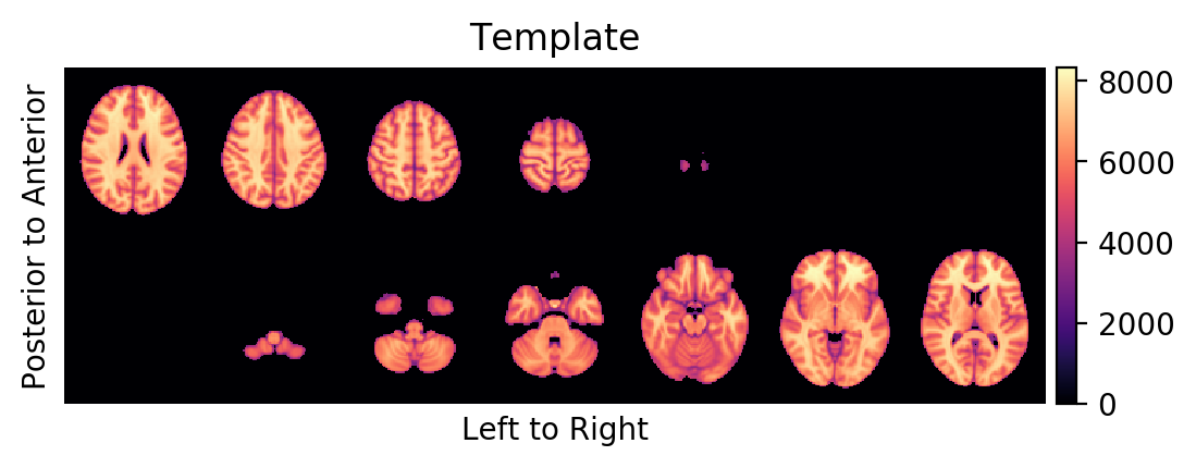
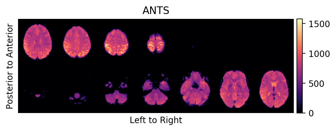
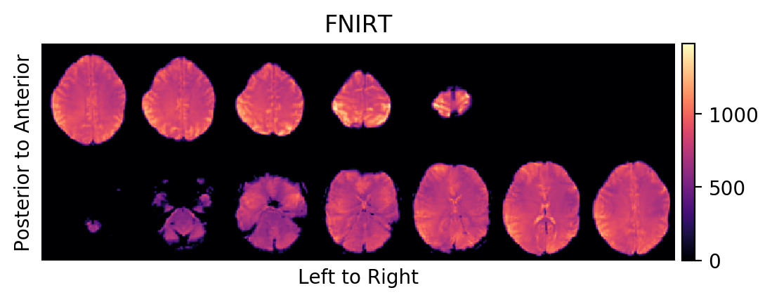
It appears that – out of the box – ANTS does a much better job in finding a suitable \(ψ\) than FNIRT (and this is true not only for this example). The brains \(r ∘ ψ\) always appear to be a bit off and too big with FNIRT. This means that when using FNIRT to fit \(ψ\), you should probably use a custom spline coefficients file and not rely on the default parameters of the algorithm.

In case you want to view the estimated images \(r∘ψ_{\text{ANTS}}\) and \(r∘ψ_{\text{FNIRT}}\) in a 3D brain volume viewer, you may want to save the images in Nifti1-format. In Python:

from fmristats.nifti import image2nii
import nibabel as ni

ni.save(image2nii(template), 'template.nii.gz')
ni.save(image2nii(popmap_ants.vb_estimate), 'template.nii.gz')
ni.save(image2nii(popmap_fnirt.vb_estimate), 'template.nii.gz')

Whether you are using ANTS, FNIRT, or a completely different software to fit \(ψ\), make sure your diffeomorphism really fits your data.

5. Fit the signal model

The command line tool fmrifit will fit a signal model to FMRI data. You will need to provide an FMRI session file (the data), a population map (a mapping from standard space to the subject reference space), and the acquisition maps (estimates of the location and tilt of the subject in the scanner during the session). Say, you have created the files:

• subject.session
• subject.rigids
• subject-mni152-ants.popmap

Then the following will fit a fully saturate, nested model (the default and recommended model in fmristats) to your FMRI:

fmrifit -v --fit subject.fit \
    --session subject.session \
    --reference-maps subject.rigids --window-radius 2 1 1 \
    --population-map subject-mni152-ants.popmap \
    --stimulus-block faces \
    --control-block shapes

In case, the foo.study file is in your path:

fmrifit -v --population-map subject-mni152-ants.popmap \
    --window-radius 2 1 1 \
    --stimulus-block faces \
    --control-block shapes

And in case, you saved the population map to subject.popmap, it is even sufficient to call:

fmrifit -v \
    --window-radius 2 1 1 \
    --stimulus-block faces \
    --control-block shapes

The above calls will all save the fit to subject.fit.

fmristats is very flexible when it comes to defining models for your data. Indeed, you have the full power of patsy at your disposal. The standard model is a nested linear model with task blocks nested in their respective task block types (here in this example within faces and shapes). In patsy-notation the model is written as:

signal ~ C(task)/C(block, Sum)

You need to provide the right hand side (the design) of the formula to fmrifit. The default call really corresponds to:

fmrifit --formula 'C(task)/C(block, Sum)' \
    --stimulus-block stimulus \
    --control-block control

If you want to model the FMRI signal as a linear model with time as a covariate:

fmrifit --formula 'C(task) + time'

An example for an insanely flexible model that may be used as an example to show the effects of over-fitting:

fmrifit --formula 'C(task) + bs(time,df=12)'

6. Remove non-brain areas

The fitting in MB estimation is done by WLS optimisation and uses a weighting scheme with non-null spatial extent. Thus, evaluating (i.e. fitting) an FMRI model close but outside of the actual brain of a subject will nevertheless result in “valid” parameter estimates. In the case that fmrifit is not supplied with a brain mask, these “outside fits” can be detected post-hoc as they are naturally accompanied by a drastic drop in available sample size.

By default, fmrifit will estimate a default data mask on \(M\) from the foreground/background difference saved in subject.session. If this mask still contains non-brain areas, you may want to further prune the parameter fields from these areas.

Prune by threshold

The command line programs fmriprune and fsl4prune can be used to generate brain masks. Both commands will force a minimum number of observations to be available around each point by either setting a user defined hard lower bound for the minimum:

fmriprune -v --threshold 2500

# or
fmriprune -v --fit subject.fit --threshold 2500

Or by setting the lower bound to a given fraction of the maximum available measurements around a point:

fmriprune -v --fraction .7

# or
fmriprune -v --fit subject.fit --fraction .7

The options --threshold and --fraction are exclusive. The default is --fraction .6842. The generated brain mask is directly saved into the file subject.fit.

Note that the mask is not actually applied to the statistic fields in subject.fit, yet. No data and no results are overwritten. You are expected to apply the mask manually.

Prune by using a wrapper to BET

The difference between fmriprune and fsl4prune is that the latter also contains a wrapper to BET:

fsl4prune -v

Defaulting to:

fsl4prune --fit subject.fit --fraction .6842 --variant R

Example: Analysing a single subject

Let us go through the analysis of a single subject study for the subject number 23 in a study called bar:

nii2image --name mni152 \
    /usr/share/data/fsl-mni152-templates/MNI152_T1_2mm_brain.nii.gz \
    vb-template.image

fmristudy -v -o bar.study \
    --vb-image vb-template.image \
    --cohort bar \
    --id 23 \
    --datetime 2017-29-04-0933 \
    --paradigm HFM \
    --single-subject yes

Instead of giving a string to --single-subject, you may also simply write »yes«. This will create some default templates for the files:

fmriinfo -v bar.study

The following code will now parse the Nifti1-file of the subject, it will run a foreground/background detection on the FMRI data, it will fit subject movements by a principal component method, and a population map using ANTS. Then it will fit the default, nested model to the FMRI by the model based estimator. After that non-brain areas are pruned from the resulting statistics field.

Create the stimulus design

fmriblock -v \
    --namex shapes \
    --onsetsx 2 84 166 248 330 \
    --durationsx 30 \
    --namey faces \
    --onsetsy 37 119 201 283 \
    --durationsy 44

Create the session data

nii2session -v --nii subject.nii.gz \
    --epi-code 3 \
    --detect-foreground -v

Estimate head movements

Fit the subject movement estimates by a principal component method:

fmririgids -v --push --cycle 42 84 102

ref2plot -v --window-radius 2 1 1

The option -p/--push will tell fmririgids to save the name of the method that has been used to estimate the rigid transformations to the study protocol in bar.study. Have a look at what has been added:

fmriinfo bar.study

Fit the diffeomorphism

Fit the diffeomorphism \(ψ\) from standard space to subject reference space.

ants4pop -vp --cycle 42 84 102

Again, the option -p/--push has been used to tell ants4pop to save the name of the method that has been used to estimate the diffeomorphism \(ψ\) from standard space to subject reference space to the study protocol in bar.study. Have a look at what has been added:

fmriinfo bar.study

Fit the model

fmrifit -v --stimulus-block faces --control-block shapes --window-radius 2 1 1

Prune non brain areas

Prune the statistics field from non-brain areas:

fsl4prune -v