Subject analysis: Inference at a single coordinate

A signal model has been fitted to FMRI session data:

fmrifit -v --stimulus-block letter --window 2 1 1 --id 2

fsl4prune -v --id 2

The Python interface will usually give you some further flexibility.

Create the model

Load the FMRI data, the head movements, and the population map from disk:

from fmristats import *

# the FMRI data
session = load(path_to_session)

# the fitted head movements (reference maps)
reference_maps = load(path_to_reference_maps)

# smooth out the movement estimates a little
reference_maps.mean(2)
reference_maps.mean(1)
reference_maps.mean(1)

# load a diffeomorphism from disk
population_map = load(path_to_population_map)

Create the model: Set the stimulus design in the model, set the MRI-observations, and set the only(!) hyperparameter of the MB-estimator, namely the curvature of the spatial weighting kernel.

model = SignalModel(
    session=session,
    reference_maps=reference_maps,
    population_map=population_map)

model.set_stimulus_design(
        s='letter',
        c='control',
        offset=5.242,
        preset=1.42)

# discard the data of the first four scan cycles
model.set_data(burn_in=4)

# set the width of the Gaussian kernel that is used for spatial
# weighting
model.set_hyperparameters('max')

AGB300-0002-WGT:
            Number of within brain observations:  2,760,279
            Number of    non brain observations: 25,502,121
            Intercept field refers to time:          165.35 s

Save the model to disk (if you like):

model.save('subject.model')

Query information

Get some information about the FMRI data:

print(session.reference.describe())
print(session.describe())
print(reference_maps.describe())

Resolution (left to right):          3.00 mm
Resolution (posterior to anterior):  3.00 mm
Resolution (inferior to superior):   4.60 mm
Diagonal of one voxel:               6.26 mm
Volume of one voxel:                41.40 mm^3
Aspect 0 on 1:                       1.00
Aspect 0 on 2:                       0.65
Aspect 1 on 2:                       0.65

EPI code: 3

Scans:        6900
Valid:        6900
Outlying:        0 (0.00%)

Scan cycles:   230
Valid:         230
Outlying:        0 (0.00%)

Get some information about the model:

print(model.describe())

Hyperparameters:
    Scale type:         max
    Factor:            3.00

Resulting in:
    Mass:            0.9973
    Scale:             2.30 mm
    FWHM:              5.42 mm
    Radius:            6.90 mm
    Diagonal:         13.80 mm

Fit the model

result = model.fit()

Save the result to disk (if you like):

result.save('subject.fit')

Prune the statistics field from non-brain areas. You are expected to do his manually, as fmristats will usually avoid deleting data:

result.mask()

Select the highest peak in the t-field

Select the highest peak in the t-statistics field:

tstatistics = result.get_field('task', 'tstatistic')

index = np.unravel_index(np.nanargmax(tstatistics.data), tstatistics.data.shape)
coordinate = tstatistics.apply_to_index(index)

print("""
    index in the image :          {}
    coordinate in standard space: {}
    hight of the peak:            {:.2f}""".format(
        index, coordinate, tstatistics.data[index]))

index in the image :          (39, 23, 40)
coordinate in standard space: [ 12. -80.   8.]
hight of the peak:            7.64

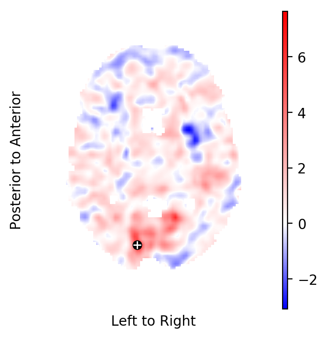
Plot the respective horizontal slice that goes through the above peak:

from fmristats.plot import picture

picture(tstatistics,3,1,1,[index[-1]],
    interpolation='bilinear', mark_peak=True)

Find out the name of standard space, so that you may use a query tool to find the region to which this coordinate belongs:

print(population_map.describe())

Population map
--------------
diffeomorphism: ants
vb:             mni152
nb:             AGB300-0002-WGT-42
vb_background:  mni152-t1
nb_background:  --
vb_estimate:    vb_estimate_ants
nb_estimate:    nb_estimate_ants
vb_mask:        --
nb_mask:        --
vb_ati:         --

Use the atlasquery tool from the FSL project to see to which structure these coordinates belong:

atlasquery -a "MNI Structural Atlas" -c 12,-80,8
MNI Structural Atlas
40% Occipital Lobe

Create a scatter plot of FMRI data around a coordinate

Extract the data at the index:

data = model.data_at_index(index).reset_index(drop=True)
print(data.iloc[:,3:].head())

   signal        time  task  block  cycle  slice    weight
0   958.0 -154.664538   0.0    0.0    7.0   11.0  0.020139
1   986.0 -154.664538   0.0    0.0    7.0   11.0  0.048931
2  1031.0 -154.664538   0.0    0.0    7.0   11.0  0.021690
3  1073.0 -154.664538   0.0    0.0    7.0   11.0  0.069630
4  1108.0 -154.664538   0.0    0.0    7.0   11.0  0.169175

Some information about the number of blocks and block labels of the stimulus design:

# Task labels
print('Task labels:               {}'.format(data.task.unique()))

# Block labels and number of blocks
print('Block labels:              {}'.format(data.block.unique()))
print('Number of blocks per task: {}'.format(len(data.block.unique())))

# Scan cycles within task blocks and their total number
print('Number of scan cycles:     {}'.format(len(data.cycle.unique())))

Task labels:               [0. 1.]
Block labels:              [0. 1. 2. 3. 4. 5. 6. 7.]
Number of blocks per task: 8
Number of scan cycles:     94

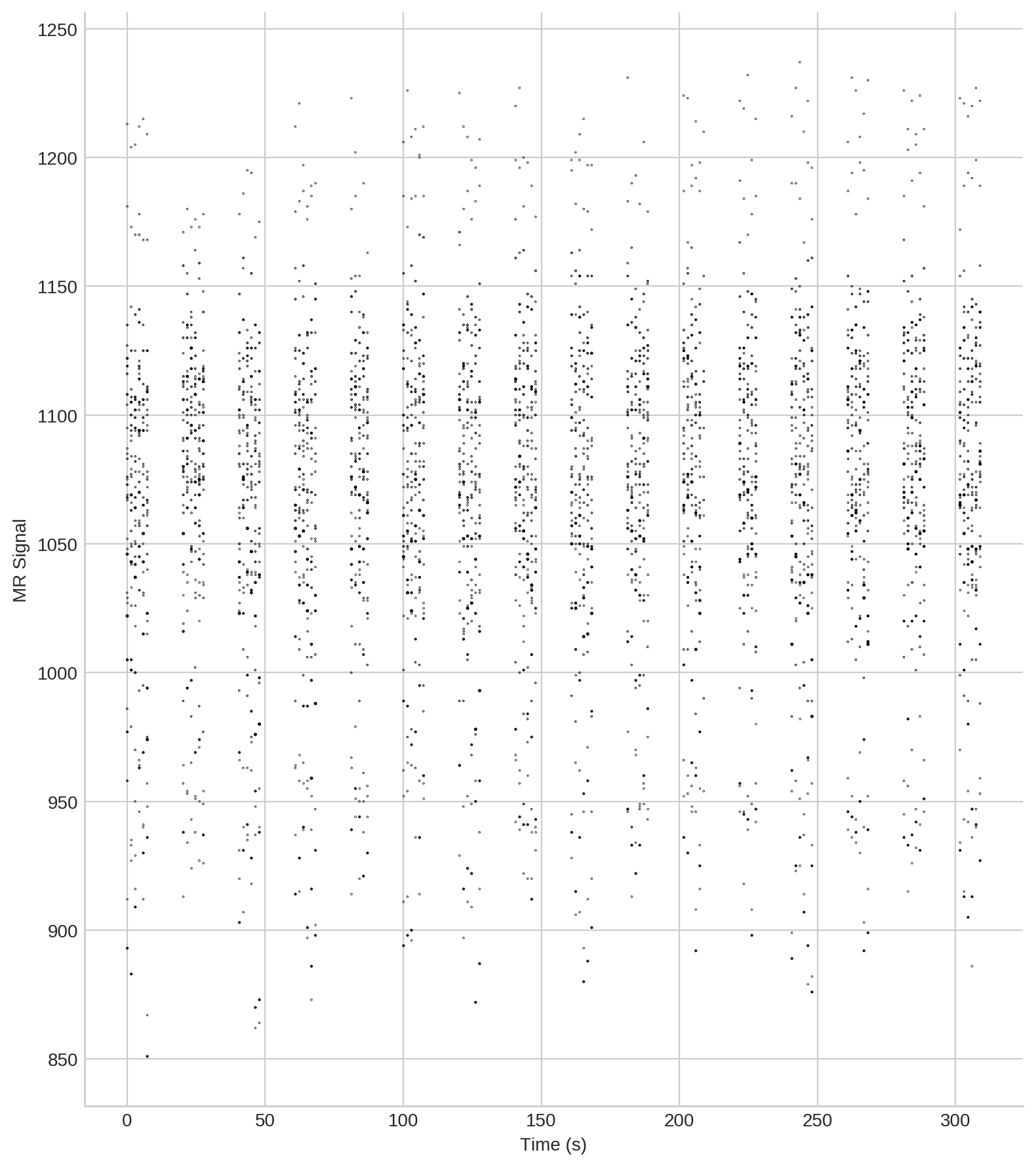
For visualisation, define a suitable scale for the scatters in relation to their distance to \(x\), and order the MRI-observations by time of acquisition:

data.time = data.time - data.time.min()
elem, idx, count = np.unique(data.time,return_index=True,return_counts=True)

w = data.weight
w = (w-w.min())/(w.max()-w.min())
w = .87*np.log(w+1.069)

Create the scatter plot (click the image to enlarge):

import matplotlib.pylab as pt
import seaborn as sb
sb.set_style('whitegrid')
pt.style.use(['seaborn-whitegrid', 'seaborn-colorblind'])

fig, ax = pt.subplots(figsize=(8,9))
ax.scatter(data.time, data.signal, s=w, marker='o', c='k')
ax.set_ylabel('MR Signal')
ax.set_xlabel('Time (s)')
sb.despine()
pt.tight_layout()

Fit different models to the data at the coordinate

fmristats is very flexible when it comes to defining models for your FMRI data. In deed, you have the full power of patsy at your disposal.

Model 1: fully saturated and nested task/block design

This is a very parsimonious and robust model for FMRI and it is the default as well as the generally recommended model when using fmristats.

fit1, model1, _ = model.fit_at_index(index,
    formula='signal~C(task)/C(block, Sum)')

data['y1'] = fit1.predict()
predict1 = fit1.predict()[idx]

Model 2: linear in time and task

This appears to be a common model. Note, however, that the model is unable to account for nested effects which typically will increase the residual mean squared error of the fit, thus, reducing your power.

fit2, model2, _ = model.fit_at_index(index,
    formula='signal~time+C(task)')

data['y2'] = fit2.predict()
predict2 = fit2.predict()[idx]

Model 3: b-spline model with 12 degrees of freedom

This model is insanely flexible and may be used as an example to show the effects of over-fitting.

fit3, model3, _ = model.fit_at_index(index,
    formula='signal~bs(time,df=12)+C(task)')

data['y3'] = fit3.predict()
predict3 = fit3.predict()[idx]

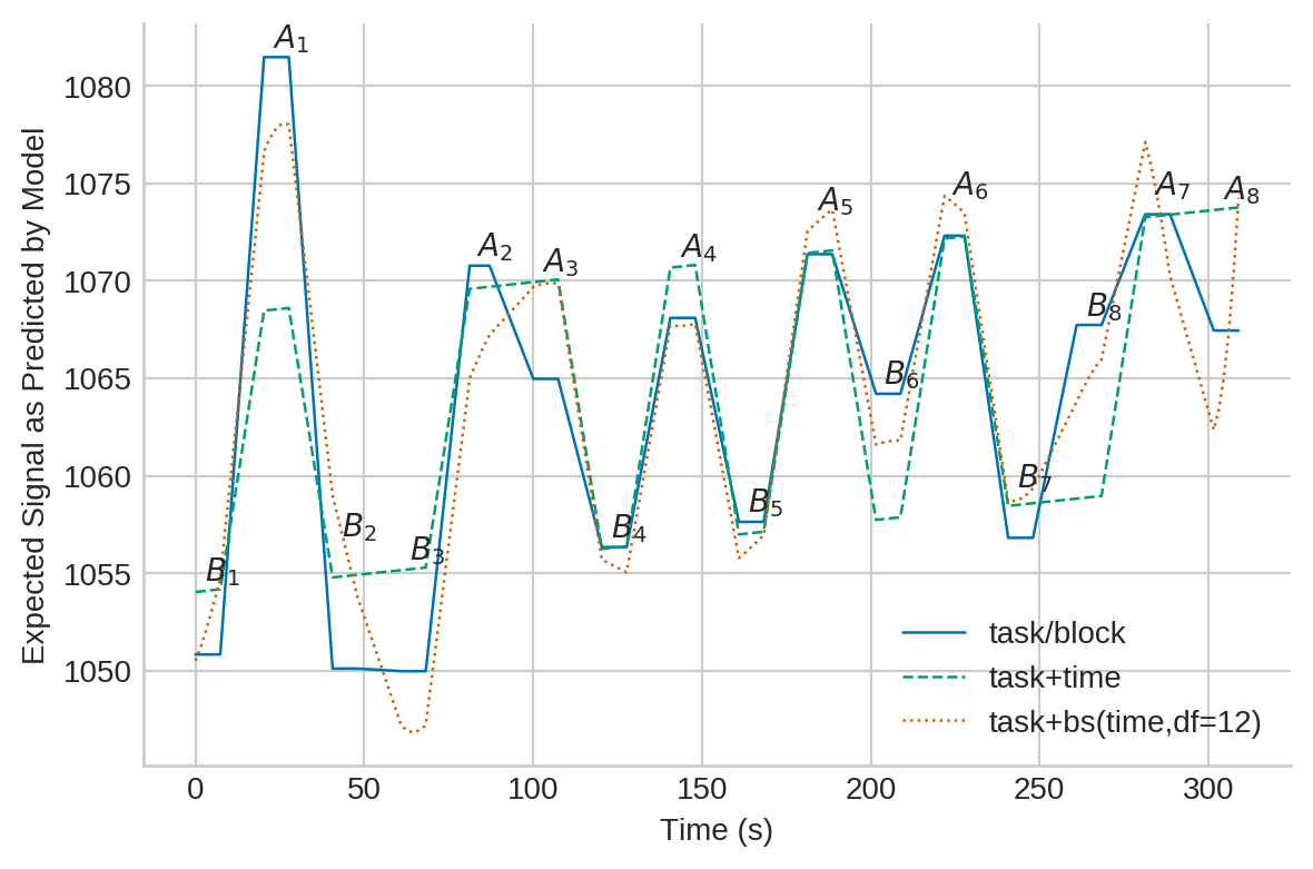
Plot the fitted regression surfaces

Plot of the fitted regression surfaces (click image to enlarge):

current_palette = sb.color_palette()
c1 = current_palette[0]
c2 = current_palette[1]
c3 = current_palette[2]

pt.close()
fig, ax = pt.subplots()
ax.plot(elem,predict1,'-',c=c1,lw=.9,label='task/block')
ax.plot(elem,predict2,'--',c=c2,lw=.9,label='task+time')
ax.plot(elem,predict3,':',c=c3,lw=.9,label='task+bs(time,df=12)')
ax.legend()
ax.set_ylabel('Expected Signal as Predicted by Model')
ax.set_xlabel('Time (s)')
sb.despine()
pt.tight_layout()

#Add block labels:
positions = data.groupby(['task', 'block']).mean()
positions = positions[['time','y1','y2','y3']]
positions.reset_index(inplace=True)
positions.set_index(['task', 'block', 'time'], inplace=True)
positions = positions.stack()
positions.index.names = ['task', 'block', 'time', 'model']
positions = positions.reset_index()
positions.set_index(['task', 'block', 'model'], inplace=True)
positions.rename(columns={0:'value'}, inplace=True)
positions.head(10)

positions = positions.reset_index()
positions = positions.groupby(['task','block','time']).max()
positions.reset_index(inplace=True)
positions.head(10)

a = fit1.params[0]
b = fit1.params[1] + a

for r in positions.itertuples():
    if np.isclose(r.task,0):
        label = r'$B_{}$'.format(int(r.block)+1)
    else:
        label = r'$A_{}$'.format(int(r.block)+1)
    ax.annotate(label, xy=(r.time-1, r.value+.5))

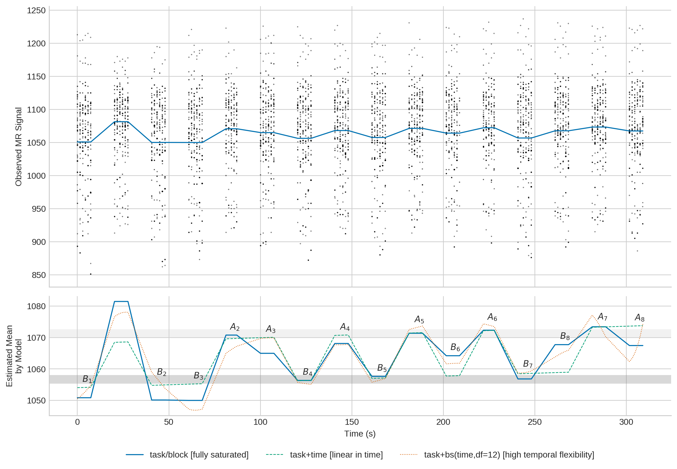
You may also combine the two plots (click image to enlarge):

figw = 11.842
figh = 5.442

figw = 11.842
figh = 7.442

a = fit1.params[0]
b = fit1.params[1] + a

left       = 0.1
right      = 0.95
maintop    = 0.99
mainbottom = 0.38
meantop    = 0.36
meanbottom = 0.1

pt.figure(figsize=(figw,figh))

# The top figure:
main_ax = pt.axes([left,mainbottom,right-left,maintop-mainbottom])
mean_ax = pt.axes([left,meanbottom,right-left,meantop-meanbottom],
    sharex=main_ax)
main_ax.scatter(data.time,data.signal,c='k',s=w,marker='o')
main_ax.set_ylabel('Observed MR Signal')
main_ax.plot(elem,predict1,'-',c=c1,lw=1.2,label='task/block')
pt.setp(main_ax.get_xticklabels(),visible=False)
sb.despine()

# The bottom figure:
mean_ax.axhline(a, c='grey', alpha=.3, lw=10)#, label='mean signal in A')
mean_ax.axhline(b, c='lightgrey', alpha=.3, lw=10)#, label='mean signal in B')
mean_ax.plot(elem,predict1,'-',c=c1,lw=1.2,
        label='task/block [fully saturated]')
mean_ax.plot(elem,predict2,'--',c=c2,lw=.8,
        label='task+time [linear in time]')
mean_ax.plot(elem,predict3,':',c=c3,lw=.8,
        label='task+bs(time,df=12) [high temporal flexibility]')
mean_ax.set_ylabel('Estimated Mean\nby Model')
mean_ax.set_xlabel('Time (s)')
mean_ax.legend(loc='lower center', bbox_to_anchor=(.5, -0.43), ncol=3)

#Add block labels:
for r in positions.itertuples():
    if np.isclose(r.task,0):
        label = r'$B_{}$'.format(int(r.block)+1)
    else:
        label = r'$A_{}$'.format(int(r.block)+1)
    mean_ax.annotate(label, xy=(r.time-1, r.value+1.8))
sb.despine()

# Save the plot to disk:
pt.savefig(scatter_plot, pad_inches=0, bbox_inches='tight')

Formal testing

Test for non-zero task related effects.

Effect strength

print(fit1.params[1])
print(fit2.params[1])
print(fit3.params[1])

14.526104774712344
14.057526450085476
13.339944081795096

Test statistic

print(fit1.tvalues[1])
print(fit2.tvalues[1])
print(fit3.tvalues[1])

7.460551272843621
7.112567149684203
4.4370014597571314

P-Values

print(fit1.pvalues[1])
print(fit2.pvalues[1])
print(fit3.pvalues[1])

1.0980615941762318e-13
1.3918174784009391e-12
9.422750022149465e-06

Test whether time is an influential factor in model 2 at this coordinate:

print(fit2.pvalues[2])

0.08344187219441945

Test whether time is an influential factor in model 2 at this coordinate:

R = np.identity(len(fit3.params))
R = R[2:,:]
print(fit3.f_test(R))

<F test: F=array([[1.9721569]]), p=0.022923767880701367,
df_denom=3273, df_num=12>

It can safely be argued that time has no significant influence, and that the data suggest no temporal signal fluctuation at \(x\). Note that even if there were, the non-parametric time dimension of model 1 would still be able to handle it.

All p-values need to be adjusted for multiple testing.