Thresholding
In Population inference: Exploratory study, we fitted a population model to the FMRI of a sample of subjects from a right-handed, healthy population that performed a word generating task. As a result, we obtained an estimate of the to-be-expected, task related BOLD effect in that population:
And we also obtained an estimate of the standard error of \(\hat β\) at each \(x∈M\), namely the field:
Now, we are interested in testing the set (or field) of hypothesis:
for every \(x∈M\) and to find areas in the brain, say \(R ⊆ M\), which contain the true and biologically relevant activations. If we reject \(H_0(x)\) at some \(x∈M\), we may say that »we can expect significant BOLD activation at \(x\) in the population«.
The set
is typically called the set of discoveries in a study.
Some notation
| \(H_0\) is accepted | \(H_0\) is rejected | Total | |
| \(H_0\) is true | \(U\) | \(V\) | \(M_0\) |
| \(H_0\) is false | \(T\) | \(S\) | \(M\setminus M_0\) |
| Total | \(R\setminus M\) | \(R\) | \(M\) |
The set \(M\) is fixed and known. The set \(M_0\) is fixed but unknown. The sets \(U,V,T,S\) and consequently also \(R\) and \(R\setminus M\) are random. We call \(R\) the discoveries in a study, and \(V\) the set of false positives. The aim is to find criteria that result in a set \(R\) such that \(R\) consists mainly of elements of \(S\) but that only contains a very limited number of elements from \(V\). To find a suitable \(R\), one studies the test statistics field:
It is custom to define \(R\) as an excursion set of the t-statistics field, i.e. to find a suitable cut-off \(t_0\) and to define
This chapter discusses different approaches for defining suitable candidates for \(t_0\).
Load statistics
Load the summary statistics from file and extract the t-test statistics field and the task related BOLD effects:
from fmristats import *
result     = load(path_to_population_result)
tstatistic = result.get_tstatistic()
bold       = result.get_parameter()
Strategies for thresholding
Nistats has some functionality that may help in detecting areas with potentially relevant BOLD activation in an image.
from nistats.thresholding import map_threshold
It is easy enough to export a fmristats’ Image-object to a
Niilike-object that Nistats can understand:
from fmristats.nifti import image2nii
tnii = image2nii(tstatistic, nan_to_zero=True)

# control the false positive rate:
_, fpr = map_threshold(tnii, level=.05, height_control='fpr')

# make a Bonferonni correction:
_, bon = map_threshold(tnii, level=.05, height_control='bonferroni')

# control the false discovery rate (Benjamini-Hochberg):
_, fdr = map_threshold(tnii, level=.05, height_control='fdr')
Let us have a look at the estimated thresholds:
print("""
Threshold (controlling FPR) : {:.2f}
Threshold (Bonferonni)      : {:.2f}
Threshold (controlling FDR) : {:.2f}""".format(
    fpr, bon, fdr))
Threshold (controlling FPR) : 1.64
Threshold (Bonferonni)      : 4.99
Threshold (controlling FDR) : 2.62
Some notes on each of the three thresholds.
False positive rate
Controlling the false positive rate (FPR) is very liberal in assigning significance to an area. The FPR is the proportion of falsely rejected \(H_0\) within the set of true \(H_0\). In signs:
(Read \(λ(V)\) as »the volume of \(V\). More precisely, \(λ\) shall denote the Lebesgue measure.) Note that the actual data you have observed don’t even play a role in the construction of the FPR-threshold; the threshold is simply identical to:
from scipy.stats.distributions import norm
print(norm.isf(0.05))
1.6448536269514729
Controlling the FPR has the effect that even when there is no activation in the brain, we would still claim \(5\%\) of the brain’s area as significant. To quote Keith Worsley: »obviously unacceptable« [2].
| [2] | The Geometry of Random Images (1996) Chance 9(1), 27-39. |
Family wise error rate
Bonferonni controls the family wise error rate (FWER) in a set of hypothesis tests. Using the notation introduced at the beginning of the chapter, the FWER is
Bonferonni’s method intrinsically depends on the »number« of hypothesis that are tested. The Bonferonni threshold accounts for this number and in our case this number is, well, infinite: The resolution at which we have evaluate the test statistics field \((t(x) : x∈M)\) is – although probably being a deliberate choice – ultimately an arbitrary choice. The resolution at which we have evaluated the \(t\)-field in this example is:
print(tstatistic.reference.describe())
Resolution (left to right):          2.00 mm
Resolution (posterior to anterior):  2.00 mm
Resolution (inferior to superior):   2.00 mm
Diagonal of one voxel:               3.46 mm
Volume of one voxel:                 8.00 mm^3
Aspect 0 on 1:                       1.00
Aspect 0 on 2:                       1.00
Aspect 1 on 2:                       1.00
But we could also have chosen a different template at a different resolution. If the resolution is increased, then so does the number of hypothesis that Bonferonni would need to account for, and so will the Bonferonni threshold. On the other hand, if we were to chose to evaluated \(t\) at a coarser resolution, the Bonferonni threshold will drop. You can see this effect by artificially dropping the resolution of the result field:
import numpy as np

def bonferroni_at_grained_image(n, level=0.05):
    data = tstatistic.data[::n,::n,::n]
    n_voxels = np.isfinite(data).sum()
    return norm.isf(level / n_voxels)

for n in range(1,6):
    print('Threshold {:n}: {:.2f}'.format(n, bonferroni_at_grained_image(n)))
Threshold 1: 4.99
Threshold 2: 4.57
Threshold 3: 4.31
Threshold 4: 4.11
Threshold 5: 3.96
The threshold drops with decreasing resolution and it will raise with increasing resolution. A threshold that depends on the resolution? Yes. Bonferonni-style thresholding of an image really makes no sense. The concept simply does not apply to a family of hypothesis of intrinsically infinite cardinality.
This does not have to be all too surprising: Let us assume that there exits at least one \(x∈M\) in the brain with true BOLD activation. Then the continuity of the test statistics field \(t\) will force the set \(R\) to have a non-trivial, positive extend around \(x\). (This is true for any threshold \(t_0\) with \(t_0<t(x)\) but also whenever \(x\) does not lie at a peak in \(t\).) But if \(R\) is not a null-set, then the probability that it contains at least one false positive can safely assumed to be \(1\). (It is unlikely that our model matches reality in such perfection that we could safely assume the opposite.) It follows indeed \(FWER=1\) almost surly – no matter how you may chose the threshold. In other words, whenever you are willing to report any area as significant, the chance of making a family error is almost surly \(1\). And to try to control an almost sure \(100\%\) at \(5\%\) really makes no sense.
False discovery rate
The false discovery rate measures the proportion of falsely rejected, true \(H_0\) among the set of discoveries \(R\). Using the above notation, the FDR equals:
Controlling the FDR – for example with Benjamini-Hochberg – does not show this strange behaviour that we have just previously seen, when feeding the method a coarser image:
from nistats.thresholding import fdr_threshold

def fdr_at_grained_image(n, level=0.05):
    data = tstatistic.data[::n,::n,::n]
    data = data[np.isfinite(data)]
    return fdr_threshold(data, level)

for n in range(1,6):
    print('Threshold {:n}: {:.2f}'.format(n, fdr_at_grained_image(n)))
Threshold 1: 2.62
Threshold 2: 2.62
Threshold 3: 2.63
Threshold 4: 2.63
Threshold 5: 2.65
As we can see, the threshold even increases mildly with decreasing resolution. If we feed less information to the procedure, the threshold is raised and not dropped. We may also expect the estimated threshold to eventually converge if the resolution of the t-statistics field increases further and to also become more accurate when supplied with more data.
Note that Benjamini-Hochberg’s procedure for controlling the FDR in \(R\) has really been constructed with having independent tests in mind. If there exists any inter-dependencies between the tests (as it is the case here), the upper bound that is produced by Benjamini-Hochberg becomes conservative. When using Bonferonni-Hochberg to control the FDR in \(R\), we can probably safely assume that the actual FDR is likely much smaller.
Get summary statistics
The FDR is usually controlled at \(1\%\) and not \(5\%\).
level         = 0.01
threshold     = fdr_threshold(tstatistic.ravel(), level)
active_volume = tstatistic.mask(tstatistic.data > threshold, inplace=False).volume()
null_volume   = level*active_volume

components, labels = tstatistic.components(threshold)

print("""
Volume claimed active:                          {:>9.2f} mm^3
Upper bound of falsely discovered volume (FDV): {:>9.2f} mm^3
Upper bound of false discovery rate (FDR):      {:>9.2f} %
Bonferonni-Hochberg threshold:                  {:>9.2f}
Components in brain claimed active:             {:>9d}""".format(
    active_volume, null_volume, 100*level, threshold, len(labels)))
Volume claimed active:                           70000.00 mm^3
Upper bound of falsely discovered volume (FDV):    700.00 mm^3
Upper bound of false discovery rate (FDR):           1.00 %
Bonferonni-Hochberg threshold:                       3.27
Components in brain claimed active:                    97
We may also chose to control the FDR at \(1\%\) and additionally force that any area claimed as active must have a minimum extend of \(100 \text{mm}^3\) (this corresponds roughly to a ball with radius \(2.88 \text{mm}\)):
# note component_size is in mm^3 and **not** in number of voxel!
components, labels = tstatistic.components(threshold, component_size=100)

active_volume = components.volume()
null_volume   = level*active_volume

print("""
Volume claimed active:                          {:>9.2f} mm^3
Upper bound of falsely discovered volume (FDV): {:>9.2f} mm^3
Upper bound of false discovery rate (FDR):      {:>9.2f} %
Bonferonni-Hochberg threshold:                  {:>9.2f}
Components in brain claimed active:             {:>9d}""".format(
    active_volume, null_volume, 100*level, threshold, len(labels)))
Volume claimed active:                           68184.00 mm^3
Upper bound of falsely discovered volume (FDV):    681.84 mm^3
Upper bound of false discovery rate (FDR):           1.00 %
Bonferonni-Hochberg threshold:                       3.27
Components in brain claimed active:                    25
Plotting fields above a threshold
import numpy as np
import matplotlib.pylab as pt
from fmristats.plot import picture
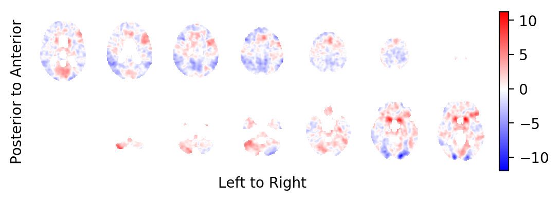
The t-statistics field:
picture(tstatistic, interpolation='bilinear')
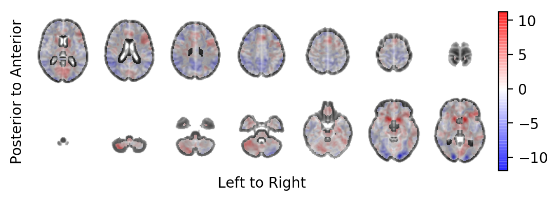
The t-statistics field with some transparency on-top of the MNI template:
picture(tstatistic, interpolation='bilinear', alpha=.6,
    background=result.model.sample.vb)
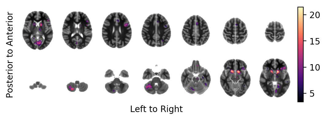
The bold effect field in ATI (in units above the template image) on-top of the MNI template in areas at which the t-tstatistic field lies above the FDR-controlled threshold and that have a minimum extent of \(100 \text{mm}^3\):
picture(bold.mask(tstatistic.data > threshold, inplace=False),
    interpolation='bilinear',
    background=result.model.sample.vb)
Effects, coordinates, locations
Thresholding a (continuous) field at a specified cut-off results in areas above the threshold which are path-wise connected components. Let us now extract (i) the highest t-statistics peak in each component, (ii) the coordinates of each peak in MNI standard space, (iii) the BOLD effect at each peak, and (iv) the structural region to which each of the peak belongs.
from scipy.ndimage import label, maximum, maximum_position

# Find the position of the highest peak within each labelled region:
peaks = maximum_position(tstatistic.data, components.data, labels)

# Find the coordinates of the peaks in MNI standard space:
coordinates = tstatistic.reference.apply_to_index(peaks)

# Get their significance (the height of the t-statistics field)
tvalues = np.array([tstatistic.data[index] for index in peaks])

# Get their task related BOLD effect
bvalues = np.array([bold.data[index] for index in peaks])
Put everything together in a nice data frame:
from pandas import DataFrame

dat = np.concatenate((peaks, coordinates,
    bvalues[:,None], tvalues[:,None]), axis=1)

df = DataFrame(dat, columns=['i', 'j', 'k', 'x', 'y', 'z', \
    'BOLD', 't_statistic'])
df.sort_values(by='t_statistic', ascending=False, inplace=True)
df.reset_index(drop=True, inplace=True)
print(df)
       i     j     k     x     y     z       BOLD  t_statistic
0   51.0  70.0  34.0 -12.0  14.0  -4.0  19.992060    11.610399
1   37.0  70.0  33.0  16.0  14.0  -6.0  20.909341    10.597062
2   29.0  33.0   8.0  32.0 -60.0 -56.0  21.198355     8.877177
3   31.0  34.0  22.0  28.0 -58.0 -28.0  13.017904     7.868119
4   65.0  77.0  35.0 -40.0  28.0  -2.0  13.077190     7.846554
5   50.0  23.0  38.0 -10.0 -80.0   4.0  10.078226     7.288186
6   69.0  37.0  27.0 -48.0 -52.0 -18.0   9.388852     7.125237
7   48.0  72.0  58.0  -6.0  18.0  44.0  10.285229     6.775694
8   61.0  56.0  25.0 -32.0 -14.0 -22.0   7.341440     5.712933
9   28.0  75.0  33.0  34.0  24.0  -6.0   8.100019     5.432309
10  42.0  56.0  31.0   6.0 -14.0 -10.0  13.418989     4.963525
11  68.0  68.0  31.0 -46.0  10.0 -10.0   7.165230     4.718494
12  75.0  47.0  34.0 -60.0 -32.0  -4.0   6.966742     4.588513
13  36.0  37.0  39.0  18.0 -52.0   6.0   7.328836     4.531171
14  60.0  31.0  54.0 -30.0 -64.0  36.0   9.316358     4.497510
15  61.0  59.0  15.0 -32.0  -8.0 -42.0   9.848705     4.442247
16  46.0  90.0  27.0  -2.0  54.0 -18.0   8.877041     4.400275
17  41.0  24.0  19.0   8.0 -78.0 -34.0   8.999326     4.288485
18  36.0  51.0  28.0  18.0 -24.0 -16.0  10.201032     4.171051
19  37.0  57.0  35.0  16.0 -12.0  -2.0   6.516204     4.038171
20  54.0  34.0  27.0 -18.0 -58.0 -18.0   6.354745     4.032904
21  48.0  82.0  26.0  -6.0  38.0 -20.0   9.863806     4.011300
22  27.0  53.0  48.0  36.0 -20.0  24.0   5.040805     3.999138
23  19.0  50.0  33.0  52.0 -26.0  -6.0   6.093332     3.918589
24  46.0  49.0  23.0  -2.0 -28.0 -26.0   8.933851     3.746942
Find the respective position of the coordinates in MNI standard space.
from subprocess import run, PIPE

def atlasquery (x, y, z):
    cmd = "atlasquery -a 'MNI Structural Atlas' -c {:f},{:f},{:f}".format(x,y,z)
    out = run([cmd], shell=True, stdout=PIPE, check=True)
    return out.stdout.decode('utf-8').strip()[31:]

df['location'] = [atlasquery(p.x,p.y,p.z) for p in df.itertuples()]

print(df.loc[:,['location','BOLD','t_statistic']])
                                 location       BOLD  t_statistic
0                             78% Caudate  19.992060    11.610399
1                 71% Putamen, 6% Caudate  20.909341    10.597062
2                         100% Cerebellum  21.198355     8.877177
3                         100% Cerebellum  13.017904     7.868119
4                        58% Frontal Lobe  13.077190     7.846554
5                      79% Occipital Lobe  10.078226     7.288186
6                       88% Temporal Lobe   9.388852     7.125237
7                        91% Frontal Lobe  10.285229     6.775694
8                       89% Temporal Lobe   7.341440     5.712933
9             66% Insula, 9% Frontal Lobe   8.100019     5.432309
10                        No label found!  13.418989     4.963525
11           29% Temporal Lobe, 5% Insula   7.165230     4.718494
12                      91% Temporal Lobe   6.966742     4.588513
13  51% Parietal Lobe, 11% Occipital Lobe   7.328836     4.531171
14                      91% Parietal Lobe   9.316358     4.497510
15                      76% Temporal Lobe   9.848705     4.442247
16                       48% Frontal Lobe   8.877041     4.400275
17                         96% Cerebellum   8.999326     4.288485
18                       3% Temporal Lobe  10.201032     4.171051
19                           32% Thalamus   6.516204     4.038171
20                         97% Cerebellum   6.354745     4.032904
21                       46% Frontal Lobe   9.863806     4.011300
22                       7% Parietal Lobe   5.040805     3.999138
23                      90% Temporal Lobe   6.093332     3.918589
24                        No label found!   8.933851     3.746942
Introducing: the FMRI fountain
In many high-throughput sciences it has become customary to visualise potential discoveries in the form of volcano plots. A volcano plot shows the observed effects (as a surrogate for the biological significance) on the x-axis and a transformation of the respective p-values of the effects (as a surrogate for statistical significance) on the y-axis. Let us create such a plot for the peaks of the t-statistics field. Note that as we are only looking »into one direction«, the plot will look more like a fountain rather than a volcano.
The following plot shows the estimated, task related BOLD effect of all peaks in the entire t-statistic field in ATI units on the x-axis, and the \(-log_{10}(p)\) of the respective p-value of this effect on the y-axis. The horizontal dashed line shows the Bonferonni-Hochberg threshold. We may assume that the proportion of false discoveries above the dashed line is below \(1\%\). The highest peak in each connected component in the FDR-thresholded image is marked by a star. The components with a minimal extent of \(100 \text{mm}^3\) are coloured.
# extract peaks of the entire field
peakmap = tstatistic.detect_peaks()

# t-values, effect estimates, and transformed p-values
all_tvalues = tstatistic.data[peakmap.data]
all_bvalues = bold.data[peakmap.data]

# transformed t-statistics
all_pt = -np.log10(norm.sf(all_tvalues))
df ['pt'] = -np.log10(norm.sf(df.t_statistic))

# height of Bonferonni-Hochberg threshold
fdrline = -np.log10(level)

pt.close()
fig, ax = pt.subplots(figsize=(8,8))
ax.axhline(fdrline, ls='--', c='k', lw=.9)
ax.scatter(all_bvalues, all_pt, marker='.', c='k')

# highest peak in each connected component
for entry in df.itertuples():
    ax.scatter(entry.BOLD, entry.pt, marker='*')

# location of top five entries in the discoveries
for entry in df[:3].itertuples():
    ax.text(entry.BOLD, entry.pt, entry.location,
        horizontalalignment='right', verticalalignment='bottom')
entry = df.iloc[3]
ax.text(entry.BOLD, entry.pt, entry.location,
    horizontalalignment='left', verticalalignment='top')
for entry in df[4:5].itertuples():
    ax.text(entry.BOLD, entry.pt, entry.location,
        horizontalalignment='right', verticalalignment='bottom')
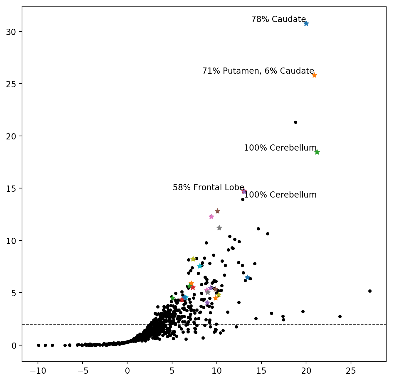
In particular the exposed position of the top right discoveries suggest high reliability.
We also see in the plot that there is a peak in the brain that shows a strong BOLD effect with high suggested statistical significance that either lies within a component that is smaller than our originally, forced \(100 \text{mm}^3\) threshold or within a component with a more prominent peak.