Population inference: Confirmation study

The analysis in Subject analysis: Inference at a single coordinate suggested that a word generating task results in a relevant and statistical significant increase in BOLD effect in the occipital lobe:

In this section, we aim to confirm this finding in a population of right-handed, healthy subjects. For right-handed, healthy subjects (with a Waterloo Handedness Score above +20) from the population have been drawn, their FMRI have been analysed, and the results collected in the file tutorial.sample:

fmrisample -v tutorial.sample \
    --covariates-query 'waterloo > 20'

Load data and fit the population model

from fmristats import *
from fmristats.plot import *

population_sample = load(path_to_sample)

print("""
    Number of subjects in total:     {:d}
    Number of right-handed subjects: {:d}
    Number of  left-handed subjects: {:d}""".format(
        len(population_sample.covariates),
        (population_sample.covariates.waterloo >= 20).sum(),
        (population_sample.covariates.waterloo <= 20).sum()))

Number of subjects in total:     64
Number of right-handed subjects: 64
Number of  left-handed subjects: 0

We are aiming to confirm a finding that has been suggested by an analysis of a single subject. Hence, remove this initial subject from the sample.

sample = population_sample.filter(population_sample.covariates.id != 2)

First, we shall have a look at the sample size per voxel in the MNI152-template (the number of subjects which have valid entries at this voxel):

sample_size = Image(
    sample.vb.reference,
    np.isfinite(sample.statistics).all(axis=-2).sum(axis=-1))

picture(sample_size.mask(inplace=False),cmap=cm.viridis)

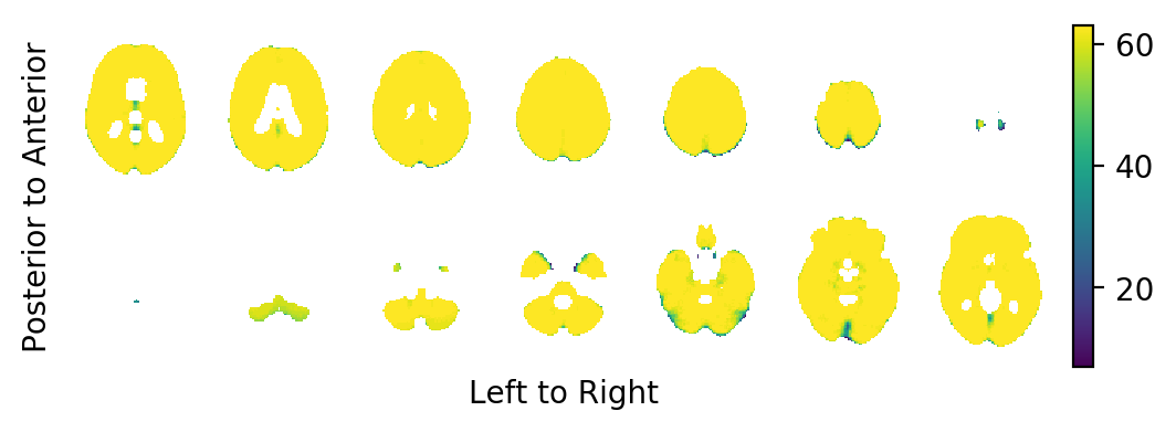
It appears that for some voxels close to the surface of the MNI152-template the population diffeomorphisms \(ψ_j\) did not fully map the template brain onto the respective subject brain. This is to be expected.

print('Sample size at the index of interest: {:.0f}'.format(
    sample_size.data[index]))

Sample size at the index of interest: 63

Let us now fit the population model (which is a random effects meta regression model in fmristats) to the sample of BOLD effects and their respective estimated standard errors:

popmod = PopulationModel(sample)
result = popmod.fit()

… not all points in the mask are identifiable.
… points with missing data along subject dimension.
… number of points to estimate: 902629
… perform a meta analysis

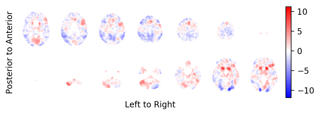
Extract the Knapp-Hartung adjusted t-statistics field

Extract the Knapp-Hartung adjusted t-statistics field that tests for non-zero, task related BOLD effects:

tstatistics = result.get_tstatistic()

picture(tstatistics)

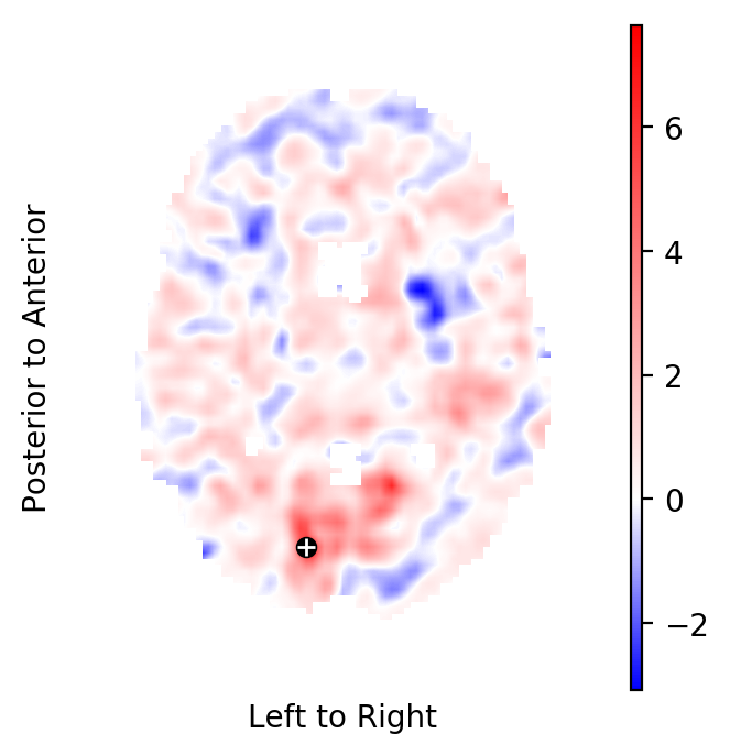
Now, plot the respective slice through the t-statistics field that has shown the above BOLD effect in the initial subject:

pt.plot([index[0]], [index[1]], 'ko')
pt.plot([index[0]], [index[1]], 'w+')
picture(tstatistics,3,1,1,[index[-1]],
    interpolation='bilinear')

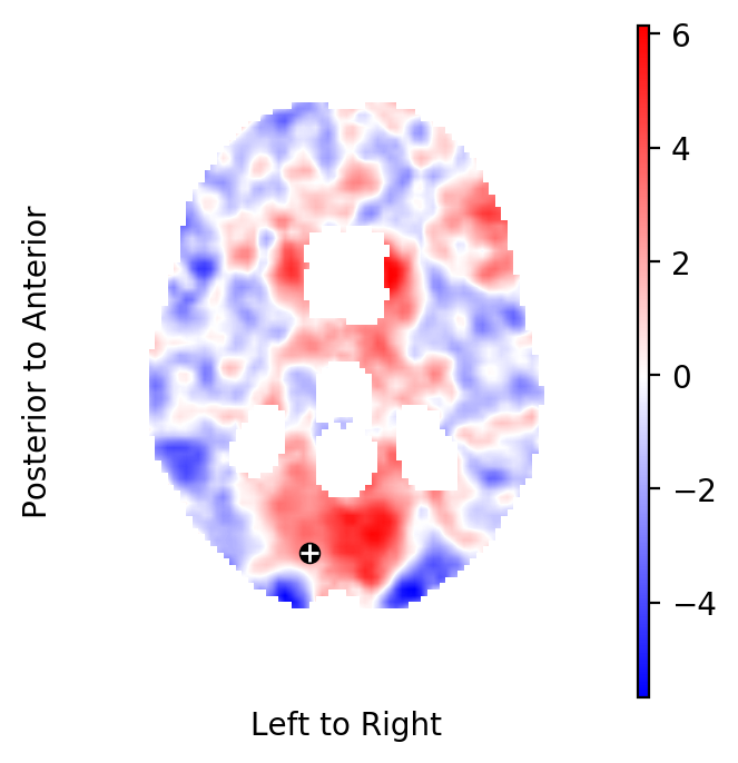
The t-statistic at these coordinates is:

print(tstatistics.data[index])

2.705125720068511

Create a forest plot of BOLD statistics

Extract the estimated BOLD effects and the respective standard errors of the estimated BOLD effects from the sample:

df = population_sample.at_index(index)
df.valid.all()
df.sort_values(by='waterloo', inplace=True)

dm = result.at_index(index)
dm.set_index('parameter', inplace=True)

Define the critical values for the plots:

from scipy.stats.distributions import t
from scipy.stats.distributions import norm

crt_subject = norm.ppf(q=.95)
crt_population = t.ppf(q=.95, df = dm.loc['Intercept', 'df'])

print(crt_subject, crt_population)

1.6448536269514722 1.669804162296528

Set some general options for the visualisation:

import matplotlib
matplotlib.rc('xtick', labelsize=8)
matplotlib.rc('ytick', labelsize=8)

import seaborn as sb
sb.set_style('whitegrid')
palette = sb.palettes.SEABORN_PALETTES['deep']

figw = 5.842
figh = 8.442

Create a forest plot in ascending order of handiness (left handed on the bottom, right handed on the top):

x = dm.loc['Intercept', 'point']
s = dm.loc['Intercept', 'stderr']

df['yvec'] = range(len(df.task))
df['waterloo'] = df.waterloo.astype(int)

fig = pt.figure(figsize=(figw,figh))
ax = pt.subplot(111)
ax.axvline(0,c='k',lw=.9, ls=':')
ax.errorbar(df.task[df.id!=2], df.yvec[df.id!=2],
    xerr=crt_subject*df.stderr[df.id!=2], fmt='o',
    label='Sample', c=palette[0])
ax.errorbar(df.task[df.id==2], df.yvec[df.id==2],
    xerr=crt_subject*df.stderr[df.id==2], fmt='o',
    label='Initial Subject', c=palette[1])
ax.errorbar(x, -1, xerr=crt_population*s, fmt='o',
    label='Population', c=palette[2])
ax.axhline(-.5,c='k',lw=.9, ls='-')
ax.set_xlabel(r'Task related BOLD effect at $x_0$ in ATI')
ax.set_ylabel('Waterloo')
ax.yaxis.set_ticks_position('none')
pt.box(False)
pt.yticks(np.hstack((df.yvec, -1)), list(df.waterloo) + ["Meta"] )
pt.legend(loc='lower center', bbox_to_anchor=(.5, -0.2), ncol=3)

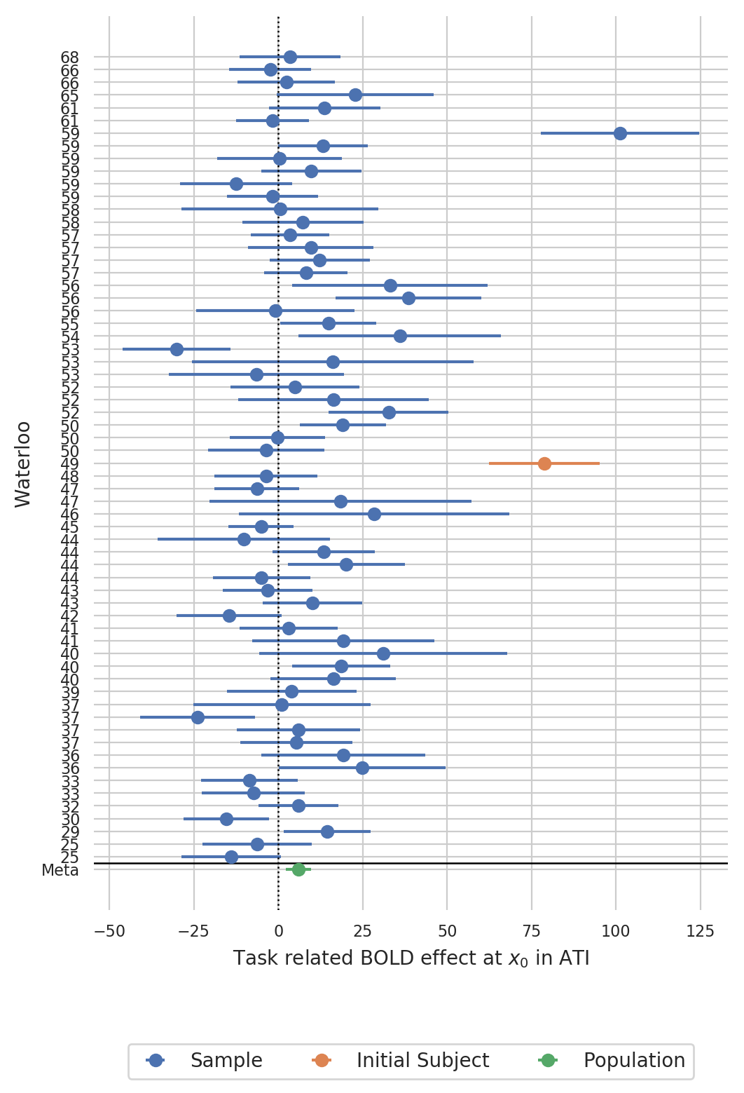
Quite interestingly, there was even one subject in the sample that showed an even larger task related BOLD effect than the initial subject at theses coordinates.

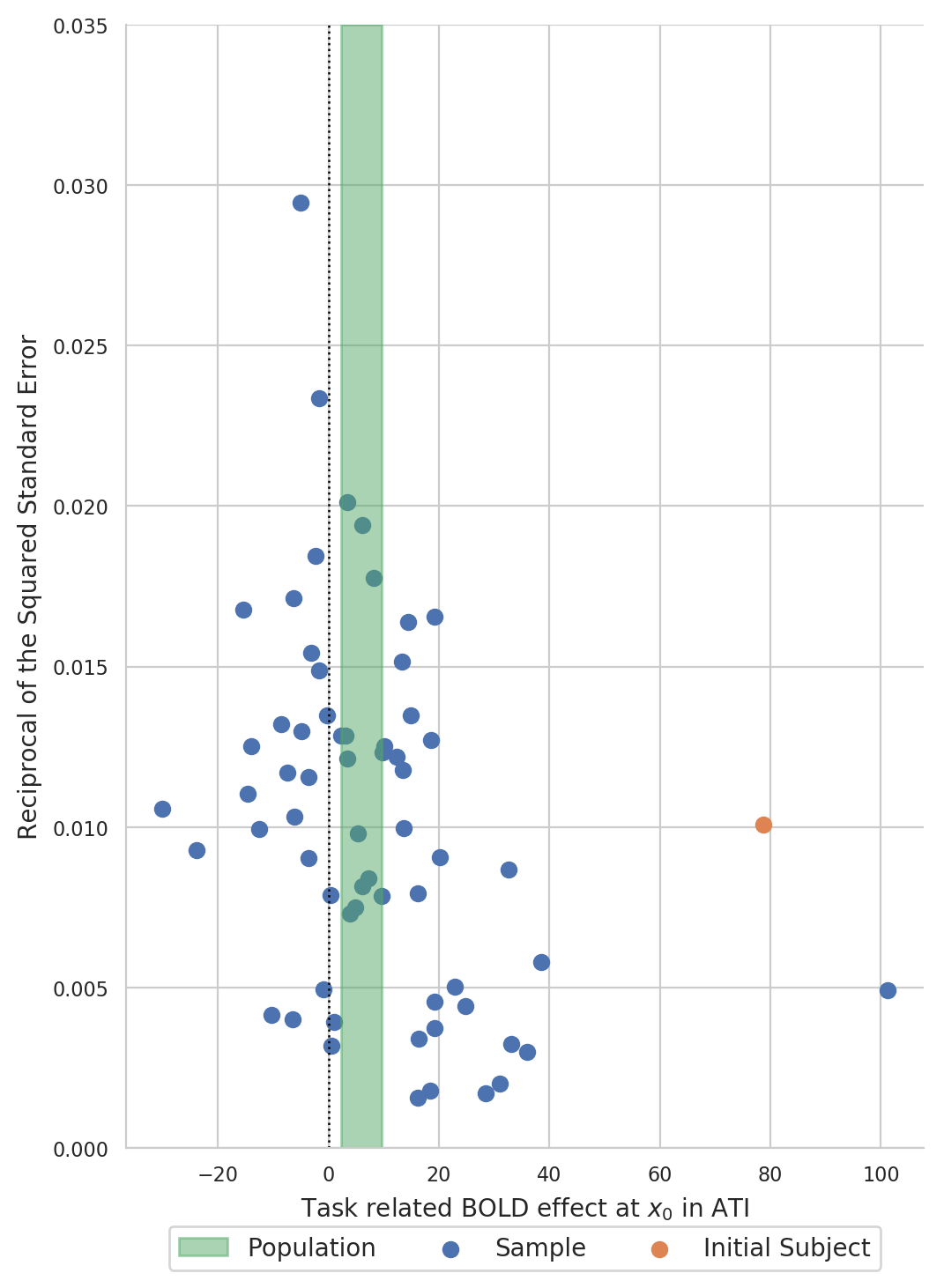
Create a funnel plot of BOLD statistics

Create a funnel plot with the estimated BOLD effect on the x-axis and the reciprocal of the squared standard error on the y-axis:

Formal testing

Any prior knowledge had been removed prior to testing the hypothesis of whether there exists a task related BOLD effect at \(x\) in the sample. Hence, there is no need to adjust for multiple testing in the inference for the population, we there was, well, no multiple testing.

Point estimate, confidence interval, and p-value of BOLD effect of the word generating task at the point \(x\) in the population:

x = dm.loc['Intercept', 'point']
s = dm.loc['Intercept', 'stderr']

print("""
Point estimate of the BOLD effect: {:.2f}
Lower bound of a 95% confidence interval: {:.2f}
Upper bound of a 95% confidence interval: {:.2f}
p-value for ≠0:                           {:.4f}""".format(
    x, x-crt_population*s, x+crt_population*s,
    dm.loc['Intercept', 'pvalue']))

Point estimate of the BOLD effect: 5.97
Lower bound of a 95% confidence interval: 2.29
Upper bound of a 95% confidence interval: 9.66
p-value for ≠0:                           0.0044

We may reject the null hypothesis that there exists no BOLD effect at \(x\) at \(1\%\) level of significance.